In this article, we will dig into fatigue life theories commonly used in practice. After learning the fundamentals of fatigue in the Introduction to Fatigue article, let’s start with the theories being used to express fatigue properties of materials.
Fatigue Life Curves
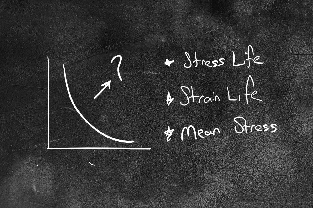
As we mentioned in the previous post that fatigue results represented in tables by Wöhler, later on, plotted in stress and life axis, and named Wöhler or SN curves. In this method, primarily elastic deformation is predominant. Failure time or cycles to failure takes a longer period. Therefore, this technique is also called high cycle fatigue and measured with stress and cycle to failure. Two different types of SN curves are discovered and schematically shown in the figure below. The graphs show that the stress life curve differs depending on the material properties.
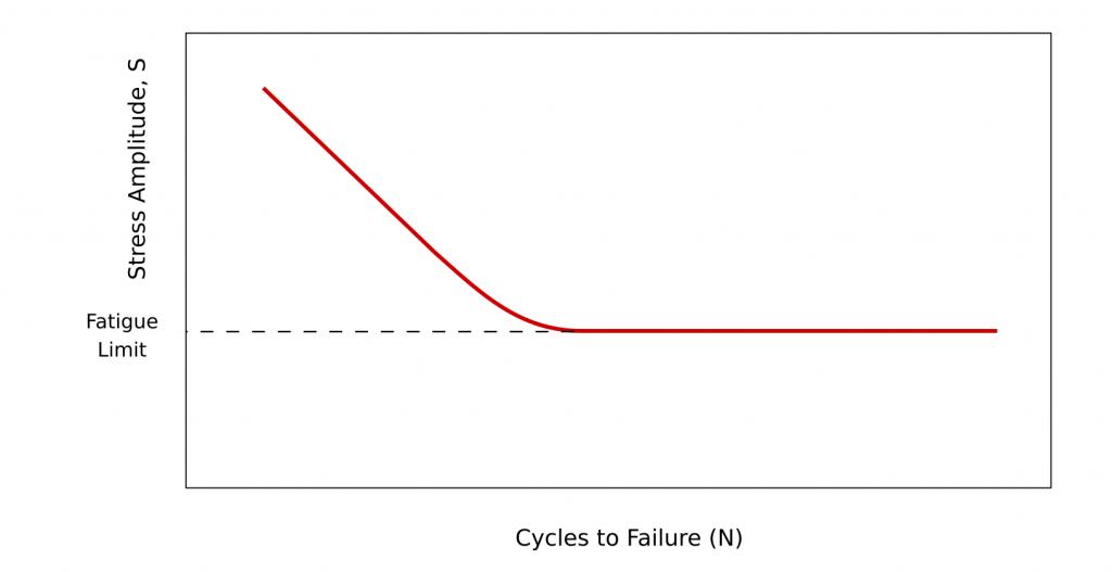
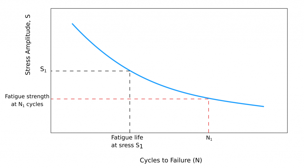
Ferrous and titanium alloys represent a fatigue limit (endurance limit). For these materials, the S-N curve becomes horizontal at higher cycles; below this line, no fatigue failure is seen for the infinite number of cycles. However, most of the non-ferrous metals show a declining trend over the cycle to failure and does not have a fatigue limit.
Another approach to fatigue life estimation is strain life. Since the failures occur in a relatively small number of cycles, it is also named low cycle fatigue. This technique is used for circumstances where fatigue loading is associated with plastic deformation (stress above the yield point). In this method, fatigue life is characterised by the strain range. In the strain life approach, the total strain has two components namely, elastic and plastic.
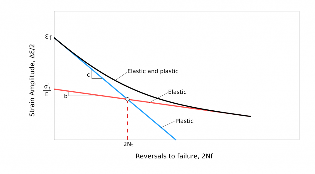
\frac{\Delta\epsilon}{2}=\Delta\epsilon_a=\underbrace{\frac{\sigma^{'}_f}{E}(2N_f)^b}_{elastic}+\underbrace{\epsilon_{f}^{'}(2N_f)^c}_{plastic}According to the plot of total strain-life, the coefficients can be listed below:
\sigma^{'}_f, fatigue strengthcoefficient \\
 \epsilon^{'}_f, fatigue ductility coefficient \\
b, fatigue strength exponent\\
c, fatigue ductility exponent\\
Understanding Mean Stress
The stress or strain life graphs above are often developed for fully reversed loading conditions where the material loaded with the ratio of -1. The mean stress is normally zero for standard developed stress-strain life graphs. However, what if you have a loading ratio different than -1 (mean stress). For these circumstances, a number of techniques were developed to find out allowable stress amplitude that your material can withstand. The most accepted methods can be listed as; Goodman, Gerber and Soderberg.
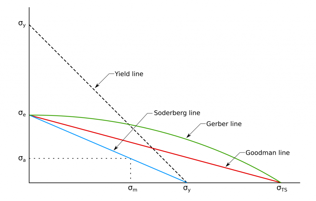
\sigma_e \text{: fatigue limit under zero mean stress} \\
\sigma_a  \text{: fatigue stress amplitude} \\
\sigma_m  \text{: mean stress} \\
\sigma_{TS}  \text{: tensile strength} \\
\sigma_{y}  \text{: yield strength} \\
Using these curves, general forms of the relationships are expressed as follows;
\sigma_a=\sigma_e(1-(\frac{\sigma_m}{\sigma_{TS}})^x)where x=1 for the Goodman line, x=2 for the Gerber line.
Soderberg expressed allowable stress amplitude under mean stress using fatigue limit and yield strength as shown below;
\sigma_a=\sigma_e(1-(\frac{\sigma_m}{\sigma_{y}}))